My Machine Learning First (Failed?) Attempt.

You can’t go anywhere or read anything today in the IT world without running into Machine Learning, it’s the hot new thing. All the cool kids are doing it, so I thought I would give it a try too. A little Python, a little Sklearn, a little SparkML, and lots of reading later…. behold my not so wonderus KMeans Unsupervised Machine Learning …… thing.
There are like a zillion articles and books about machine learning out there, most of them surprisingly unhelpful. I even bought a few on my Kindle, I usually made it about 3 chapters before my eyes started to glaze over. Either too much theory and math that seems totally pointless because some ML library does it for you, or on the other end of the spectrum, just a bunch of code that looks like it’s doing something with little to no explanation. It’s been impossible to find something in the middle ground. Here is what I have learned approaching the subject as someone who always wants to be a data engineer and never a data scientist. All the code for this is on Github.
- Get a general understanding of the basic algorithms available in most ML libraries.
- Try to learn which algorithms and approaches work for which kind of problems.
- Learn and understand the data you are working with first.
- Feature engineering … aka selection and scaling etc of the variables you will feed into your model.
- See what happens.
Let’s jump in. First, one of the easiest machine learning algorithms to implement is called Kmeans. It’s basically a way of looking at unlabeled data and clustering data points together based on the feature inputs. So think of customer segmentation. My first thought was go back to the ye ole’ Lending Tree free data sets. I knew it had a lot of numeric values about the people that got loans. If I was Lending Tree and a prospective client was filling out a form and gave me their Income and Age for example, could I use Machine Learning to put them into a segment or group and maybe know something about their possible interest rate they might get before hand?
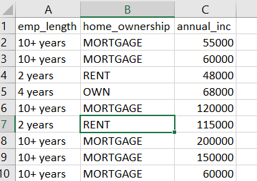
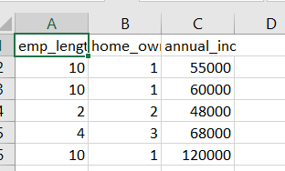
The data set I downloaded for a single quarter is 128,000 records. For my features I selected Employment Length, Income, and Home Ownership. As you can see some of the features will need to be converted to numeric. Mortgage will be 1, Rent will be 2, Own 3. Should look like below when you’re done. I have no idea if this is was a good idea or not.
Next I need to find the K, or number of clusters to feed to Spark, I will plot with scikit-learn, but needed to scale the features first. We do this to make sure all the inputs will be treated the same, they need to be of the same scale. You can imagine on a graph if you are trying to plot something that is 1 vs 20, it just isn’t going to work out. Luckily scikit-learn has something called a StandardScaler to help us with this.
We can use .fit() to calculate the mean and std to be used, then call .transform() , giving us our features scaled. Or just use .fit_transform() and do both!
import pandas as pd
from sklearn.preprocessing import StandardScaler
from sklearn.cluster import KMeans
import matplotlib.pyplot as plt

data = pd.read_csv('loanfeatures.csv')
scaler = StandardScaler()
scaled_data = scaler.fit_transform(data)

df = pd.DataFrame.from_dict(scaled_data)

print(df.head())The next problem with the Kmeans approach is the K part. K being the number of clusters, how do we know what the optimum number of clusters to use is? Below is what I did, took awhile to run on my laptop. The idea is to find the elbow of the plot. I followed this great tutorial.
squared_distances_sumof = []
K = range(1,15)
for k in K:
    km = KMeans(n_clusters=k)
    km = km.fit(scaled_data)
    squared_distances_sumof.append(km.inertia_)

plt.plot(K, squared_distances_sumof, 'bx-')
plt.xlabel('k')
plt.ylabel('Sum_of_squared_distances')
plt.title('Elbow Method For Optimal k')
plt.show()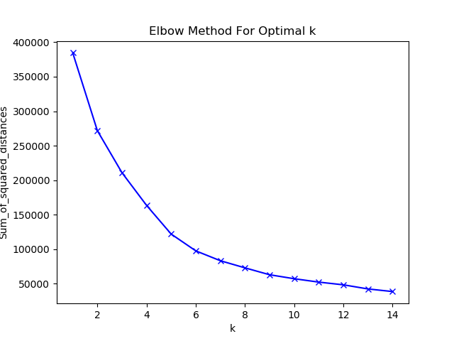
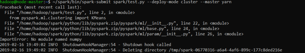
OK, now time to switch to Spark! I’ve got a 3 node setup running Hadoop YARN, with my Spark integrated to run inside my YARN cluster. Here is a simple example of reading my csv file I stored in Hadoop into a Spark dataframe and printing out the top 20 records. (Spark 2.4)
~/spark/bin/spark-submit spark/test.py --deploy-mode cluster --master yarnfrom pyspark.sql import SparkSession
spark = SparkSession.builder.appName('test machine learning').getOrCreate()
df = spark.read.load("hdfs://node-master:9000/loanfeatures.csv", format="csv", sep=":", inferSchema="true", header="true")
df.show()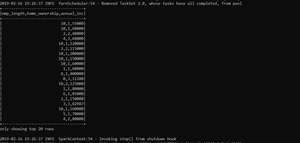
Uh oh. First problem. So when working with PySpark in a YARN settings, either you must package up the needed python dependencies in a zip and submit them at job time to be distributed, which isn’t possible with numpy because of it’s C dependencies. The only other option is to install what you need on each worker node. (or use Scala)
Here is the full code. We can step through it, pretty straight forward.
from pyspark.sql import SparkSession, SQLContext
from pyspark.ml.clustering import KMeans
from pyspark.ml.feature import VectorAssembler, StandardScaler
from pyspark.sql.functions import monotonically_increasing_id
import pandas as pd


spark = SparkSession.builder.appName('test machine learning').getOrCreate()
sqlContext = SQLContext(spark)

df = spark.read.load("loanfeatures.csv", format="csv", sep=",", inferSchema="true", header="true")
df_no_nulls = df.na.drop()
df_id = df_no_nulls.withColumn("id", monotonically_increasing_id())

assembler = VectorAssembler(inputCols=["emp_length", "home_ownership", "annual_inc"],outputCol="features")

output = assembler.transform(df_id)
output = output.select("id","features")
scaler = StandardScaler(inputCol="features", outputCol="scaledFeatures", withStd=True, withMean=True)

scalerModel = scaler.fit(output)
scaledData = scalerModel.transform(output)
dataframe = scaledData.select("id","scaledFeatures")

k = 7
kmeans = KMeans().setK(k).setSeed(1).setFeaturesCol("scaledFeatures")
model = kmeans.fit(dataframe)
centers = model.clusterCenters()

transformed = model.transform(dataframe).select('id', 'prediction')
rows = transformed.collect()
new_df = sqlContext.createDataFrame(rows)
df_pred = new_df.join(dataframe, 'id')
pandaDf = df_pred.toPandas()
pandaDf.to_csv('results.csv', sep=',', encoding='utf-8')
spark.stop()
First, using PySpark, a SQLContext is a easy choice, makes reading things like CSV files into Data Frames easy. ( What I’m doing here is only possible in version 2.2+ of Spark.
spark = SparkSession.builder.appName('test machine learning').getOrCreate()
sqlContext = SQLContext(spark)
df = spark.read.load("loanfeatures.csv", format="csv", sep=",", inferSchema="true", header="true")
Next, I’m just working the data. Dropping any NULLs and adding a Id column using a Spark function called monotonically_increasing_id()
df_no_nulls = df.na.drop()
df_id = df_no_nulls.withColumn("id", monotonically_increasing_id())
Of course there is always a catch, Kmeans in Spark requires Vectors. So we have to transform our Data Frame. If you print it, it basically appears as a single column with what looks like a Python list.
assembler = VectorAssembler(inputCols=["emp_length", "home_ownership", "annual_inc"],outputCol="features")

output = assembler.transform(df_id)
output = output.select("id","features")
Just like before, we must Scale the features now. Below you can see the scaled features and the vector column that holds them.
scaler = StandardScaler(inputCol="features", outputCol="scaledFeatures", withStd=True, withMean=True)

scalerModel = scaler.fit(output)
scaledData = scalerModel.transform(output)
dataframe = scaledData.select("id","scaledFeatures")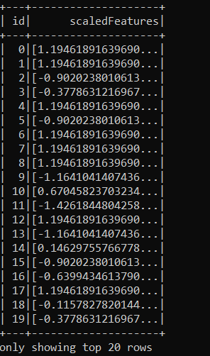
After we have our scaled features, next is the magic.
k = 7
kmeans = KMeans().setK(k).setSeed(1).setFeaturesCol("scaledFeatures")
model = kmeans.fit(dataframe)
centers = model.clusterCenters()

transformed = model.transform(dataframe).select('id', 'prediction')
Finally, we have what we need. I join back to the original data set, and use Pandas to export the results. You can see the output below along with the model prediction.
rows = transformed.collect()
new_df = sqlContext.createDataFrame(rows)
df_pred = new_df.join(dataframe, 'id')
pandaDf = df_pred.toPandas()
pandaDf.to_csv('results.csv', sep=',', encoding='utf-8')
spark.stop()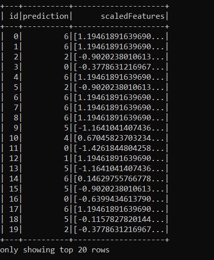
The code to generate the plot of the results is short and sweet.
import pandas as pd
import matplotlib.pyplot as plt
from mpl_toolkits.mplot3d import Axes3D

df = pd.read_csv('results.csv')

threedee = plt.figure(figsize=(12,10)).gca(projection='3d')
threedee.scatter(df.x, df.y, df.z, c=df.prediction)
threedee.set_xlabel('x')
threedee.set_ylabel('y')
threedee.set_zlabel('z')
plt.show()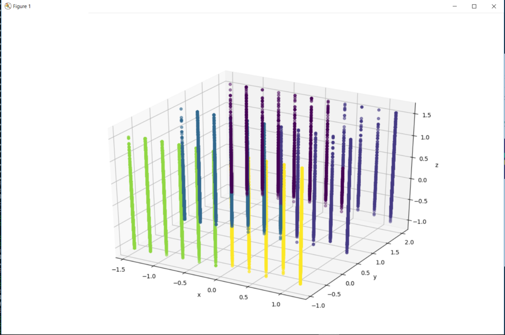
Well, that isn’t what I was expecting. I was looking for a 3d plot of clusters. Slightly confusing that different clusters are appearing on straight lines, with the data points stacked. I mean obviously there are different clusters. Not sure what went wrong, maybe I will try again with a different smaller data set. It was fun to walk through a at least an attempt at machine learning. One step at a time, that’s how I learn!