Geospatial Data with Apache Spark – Intro to RasterFrames

Yikes, distributed geospatial data processing at scale. That has fun written all over it… not. There isn’t that many people doing it so StackOverflow isn’t that useful. Anyone who has been around geospatial data knows the tools like GDAL are notoriously hard to use and buggy… and that one’s probably the “best.” What to do when you want to process and explore large satellite datasets like Landsat and Modis? Terrabytes/petabytes of data, what are going to do, download it? The power of distributed processing with Apache Spark. The simplicity of using SQL to work on geospatial data. Put them together… rasterframes. What a beast.
Why use RasterFrames on Apache Spark?
It’s important to think about the basics here. Of course anything geospatial is “custom”, tools like Spark don’t come with out of the box complex spatial support. Why would anyone want to use something like RasterFrames on top of Apache Spark? Full code set available on GitHub.
- Big data processing is hard and complex, Apache Spark hides most of that complexity away.
- Geospatial processing is even harder, RasterFrames provides APIs to apply common geospatial functions to data.
- RasterFrames provides “catalogs” on-top of well known satellite imagery like Modis and Landsat.
- You don’t have to download terra-bytes of data locally.
- You can use SQL to interact with geospatial data, easy to understand and less complex than custom code.
I’m going to be using my 3 node Spark cluster I setup and recently talked about. Next I have to go about getting my Spark cluster installed with RasterFrames and the tools it relies on.
Installing RasterFrames and its dependencies on an Apache Spark cluster.
Install GDAL on Spark Nodes and Master.
On each one of the Spark nodes we first install GDAL. This the library used behind the scene to read geospatial raster tifs.
sudo apt-get install python3.6-dev
sudo add-apt-repository ppa:ubuntugis/ppa && sudo apt-get update
sudo apt-get update
sudo apt-get install gdal-bin
sudo apt-get install libgdal-dev
export CPLUS_INCLUDE_PATH=/usr/include/gdal
export C_INCLUDE_PATH=/usr/include/gdal
pip3 install GDAL==2.4.2
Install pyRasterFrames and run some code.
Next we pip install pyrasterframes on all our nodes.
$ python3 -m pip install pyrasterframesFinally we can start playing with rasterframes. On my Spark master I change directories into where I will submit my pyspark programs…
cd /usr/local/spark/bin/Next I download the python source zip for rasterframes… this is needed as an argument for the pyspark command.
curl https://repo1.maven.org/maven2/org/locationtech/rasterframes/pyrasterframes_2.11/0.9.0/pyrasterframes_2.11-0.9.0-python.zip --output pyrasterframes_2.11-0.9.0-python.zipFinally, I tried to drop into a local PySpark session….
pyspark --master local[*] --py-files pyrasterframes_2.11-0.9.0-python.zip --packages org.locationtech.rasterframes:rasterframes_2.11:0.9.0,org.locationtech.rasterframes:pyrasterframes_2.11:0.9.0,org.locationtech.rasterframes:rasterframes-datasource_2.11:0.9.0 --conf spark.serializer=org.apache.spark.serializer.KryoSerializer --conf spark.kryo.registrator=org.locationtech.rasterframes.util.RFKryoRegistrator --conf spark.kryoserializer.buffer.max=500mFlipping random Java error. I’ve played enough with Spark and Hadoop not to be surprised by this, never fails. Typically the first thing I try is just go find the missing JAR somewhere on the interwebs and put it where it needs to be.
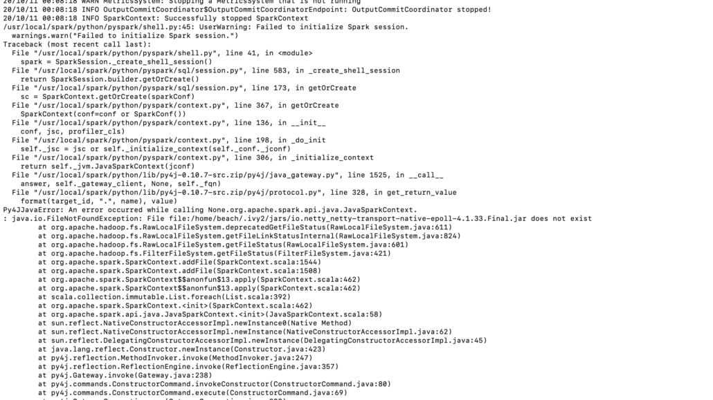
In my case the following lines of code fixed the problem. I call that a partial success when you can get these strange tools installed and the PySpark session up and running!
cd /home/beach/.ivy2/jars/
curl https://repo1.maven.org/maven2/io/netty/netty-transport-native-epoll/4.1.33.Final/netty-transport-native-epoll-4.1.33.Final.jar --output io.netty-transport-native-epoll-4.1.33.Final.jar
cp io.netty-transport-native-epoll-4.1.33.Final.jar io.netty_netty-transport-native-epoll-4.1.33.Final.jar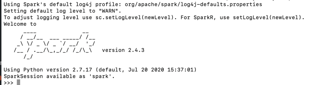
Diving into RasterFrames via Python.
Ok, now we can actually dive into the hard part, writing some geospatial code that runs on Spark! First, lets make sure that rasterframes is even working at all using the into quickstart example.
import pyrasterframes
spark = spark.withRasterFrames()
df = spark.read.raster('https://landsat-pds.s3.amazonaws.com/c1/L8/158/072/LC08_L1TP_158072_20180515_20180604_01_T1/LC08_L1TP_158072_20180515_20180604_01_T1_B5.TIF')
print(df.head())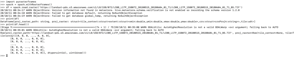
Looks like we got some array going on there, so let’s call it good. Now let’s try something a little more fun!
Basic RasterFrames concepts.
- raster – basically an array/dataframe/grid of values that represent and image.
- cell – one of the values from above.
- scene – a geospatial area of a raster, for a specific date, with a corresponding CRS.
- tile – a piece of the above scene
The power of RasterFrames catalogs.
Here is a basic overview of the rasterframes catalogs, basically all the satellite information at our DataFrame finger tips! The initial load of the catalog will take a minute or two, but be cached after that. It’s super easy to load the Landsat8 catalog into a dataframe and see the schema. You can see from the below columns we now have access to all the Landsat data that we can easily filter down to what we need.
import pyrasterframes
spark = spark.withRasterFrames()
from pyspark.sql import SQLContext
sqlc = SQLContext(spark)

l8 = spark.read.format('aws-pds-l8-catalog').load()
l8.printSchema()

// ouput
|-- product_id: string (nullable = false)
 |-- entity_id: string (nullable = false)
 |-- acquisition_date: timestamp (nullable = false)
 |-- cloud_cover_pct: float (nullable = false)
 |-- processing_level: string (nullable = false)
 |-- path: short (nullable = false)
 |-- row: short (nullable = false)
 |-- bounds_wgs84: struct (nullable = false)
 |    |-- xmin: double (nullable = false)
 |    |-- ymin: double (nullable = false)
 |    |-- xmax: double (nullable = false)
 |    |-- ymax: double (nullable = false)
 |-- B1: string (nullable = true)
 |-- B2: string (nullable = true)
 |-- B3: string (nullable = true)
 |-- B4: string (nullable = true)
 |-- B5: string (nullable = true)
 |-- B6: string (nullable = true)
 |-- B7: string (nullable = true)
 |-- B8: string (nullable = true)
 |-- B9: string (nullable = true)
 |-- B10: string (nullable = true)
 |-- B11: string (nullable = true)
 |-- BQA: string (nullable = true)


print(l8.head())
// output
20/10/11 02:06:36 WARN CSVDataSource: CSV header does not conform to the schema.
CSV file: file:///home/beach/.rf_cache/scene_list-35bc8c4913b62c16282cb33dde3e533f.gz
Row(product_id='LC08_L1TP_033037_20130318_20170310_01_T1', entity_id='LC80330372013077LGN02', acquisition_date=datetime.datetime(2013, 3, 18, 17, 42, 46, 110000), cloud_cover_pct=32.08000183105469, processing_level='L1TP', path=33, row=37, bounds_wgs84=Row(xmin=-108.24641, ymin=32.13761, xmax=-105.78492, ymax=34.15855), B1='https://s3-us-west-2.amazonaws.com/landsat-pds/c1/L8/033/037/LC08_L1TP_033037_20130318_20170310_01_T1/LC08_L1TP_033037_20130318_20170310_01_T1_B1.TIF', B2='https://s3-us-west-2.amazonaws.com/landsat-pds/c1/L8/033/037/LC08_L1TP_033037_20130318_20170310_01_T1/LC08_L1TP_033037_20130318_20170310_01_T1_B2.TIF', B3='https://s3-us-west-2.amazonaws.com/landsat-pds/c1/L8/033/037/LC08_L1TP_033037_20130318_20170310_01_T1/LC08_L1TP_033037_20130318_20170310_01_T1_B3.TIF', B4='https://s3-us-west-2.amazonaws.com/landsat-pds/c1/L8/033/037/LC08_L1TP_033037_20130318_20170310_01_T1/LC08_L1TP_033037_20130318_20170310_01_T1_B4.TIF', B5='https://s3-us-west-2.amazonaws.com/landsat-pds/c1/L8/033/037/LC08_L1TP_033037_20130318_20170310_01_T1/LC08_L1TP_033037_20130318_20170310_01_T1_B5.TIF', B6='https://s3-us-west-2.amazonaws.com/landsat-pds/c1/L8/033/037/LC08_L1TP_033037_20130318_20170310_01_T1/LC08_L1TP_033037_20130318_20170310_01_T1_B6.TIF', B7='https://s3-us-west-2.amazonaws.com/landsat-pds/c1/L8/033/037/LC08_L1TP_033037_20130318_20170310_01_T1/LC08_L1TP_033037_20130318_20170310_01_T1_B7.TIF', B8='https://s3-us-west-2.amazonaws.com/landsat-pds/c1/L8/033/037/LC08_L1TP_033037_20130318_20170310_01_T1/LC08_L1TP_033037_20130318_20170310_01_T1_B8.TIF', B9='https://s3-us-west-2.amazonaws.com/landsat-pds/c1/L8/033/037/LC08_L1TP_033037_20130318_20170310_01_T1/LC08_L1TP_033037_20130318_20170310_01_T1_B9.TIF', B10='https://s3-us-west-2.amazonaws.com/landsat-pds/c1/L8/033/037/LC08_L1TP_033037_20130318_20170310_01_T1/LC08_L1TP_033037_20130318_20170310_01_T1_B10.TIF', B11='https://s3-us-west-2.amazonaws.com/landsat-pds/c1/L8/033/037/LC08_L1TP_033037_20130318_20170310_01_T1/LC08_L1TP_033037_20130318_20170310_01_T1_B11.TIF', BQA='https://s3-us-west-2.amazonaws.com/landsat-pds/c1/L8/033/037/LC08_L1TP_033037_20130318_20170310_01_T1/LC08_L1TP_033037_20130318_20170310_01_T1_BQA.TIF')
Let’s use our SQL context to create a table of this data frame. SQL is so nice and easy to work with! Let’s do a fun little Midwest project.. We will need the Red (band 4) and NIR (band 5) bands. We will also need to mask/cutout a small geometry from where I’ve seen downed corn from around my area. The event was around August 10-11th timeframe.
sqlc.registerDataFrameAsTable(l8, "landsat_catalog")
df2 = sqlc.sql("""SELECT product_id, entity_id, acquisition_date, B4, B5, st_geometry(bounds_wgs84) as geom, bounds_wgs84
                FROM landsat_catalog
                WHERE acquisition_date > to_date('2020-08-01') AND acquisition_date < to_date('2020-08-31')
""")
df2.show()
// output
+--------------------+--------------------+--------------------+--------------------+--------------------+--------------------+
|          product_id|           entity_id|    acquisition_date|                  B4|                  B5|                geom|
+--------------------+--------------------+--------------------+--------------------+--------------------+--------------------+
|LC08_L1TP_141013_...|LC81410132020214L...|2020-08-01 04:37:...|https://s3-us-wes...|https://s3-us-wes...|POLYGON ((100.400...|
|LC08_L1TP_141027_...|LC81410272020214L...|2020-08-01 04:42:...|https://s3-us-wes...|https://s3-us-wes...|POLYGON ((89.7727...|
|LC08_L1TP_141035_...|LC81410352020214L...|2020-08-01 04:45:...|https://s3-us-wes...|https://s3-us-wes...|POLYGON ((86.3293...|
|LC08_L1TP_221068_...|LC82210682020214L...|2020-08-01 13:13:...|https://s3-us-wes...|https://s3-us-wes...|POLYGON ((-48.016...|
|LC08_L1TP_004068_...|LC80040682020214L...|2020-08-01 14:52:...|https://s3-us-wes...|https://s3-us-wes...|POLYGON ((-72.736...|
|LC08_L1TP_180047_...|LC81800472020215L...|2020-08-02 08:51:...|https://s3-us-wes...|https://s3-us-wes...|POLYGON ((21.8866...|
|LC08_L1TP_228234_...|LC82282342020215L...|2020-08-02 15:02:...|https://s3-us-wes...|https://s3-us-wes...|POLYGON ((79.0523...|
|LC08_L1TP_027245_...|LC80272452020215L...|2020-08-02 18:25:...|https://s3-us-wes...|https://s3-us-wes...|POLYGON ((-31.590...|
|LC08_L1TP_123010_...|LC81230102020216L...|2020-08-03 02:44:...|https://s3-us-wes...|https://s3-us-wes...|POLYGON ((132.802...|
|LC08_L1TP_187043_...|LC81870432020216L...|2020-08-03 09:33:...|https://s3-us-wes...|https://s3-us-wes...|POLYGON ((12.3517...|
|LC08_L1TP_203234_...|LC82032342020216L...|2020-08-03 12:28:...|https://s3-us-wes...|https://s3-us-wes...|POLYGON ((117.548...|
|LC08_L1TP_018046_...|LC80180462020216L...|2020-08-03 16:10:...|https://s3-us-wes...|https://s3-us-wes...|POLYGON ((-87.493...|
|LC08_L1TP_130022_...|LC81300222020217L...|2020-08-04 03:32:...|https://s3-us-wes...|https://s3-us-wes...|POLYGON ((109.654...|
|LC08_L1TP_146019_...|LC81460192020217L...|2020-08-04 05:10:...|https://s3-us-wes...|https://s3-us-wes...|POLYGON ((87.0921...|
|LC08_L1TP_009025_...|LC80090252020217L...|2020-08-04 15:06:...|https://s3-us-wes...|https://s3-us-wes...|POLYGON ((-65.195...|
|LC08_L1TP_025247_...|LC80252472020217L...|2020-08-04 18:13:...|https://s3-us-wes...|https://s3-us-wes...|POLYGON ((-48.257...|
|LC08_L1TP_169064_...|LC81690642020218L...|2020-08-05 07:50:...|https://s3-us-wes...|https://s3-us-wes...|POLYGON ((33.6041...|
|LC08_L1TP_201039_...|LC82010392020218L...|2020-08-05 10:58:...|https://s3-us-wes...|https://s3-us-wes...|POLYGON ((-7.8563...|
|LC08_L1TP_048002_...|LC80480022020218L...|2020-08-05 18:58:...|https://s3-us-wes...|https://s3-us-wes...|POLYGON ((-84.825...|
|LC08_L1TP_096084_...|LC80960842020219L...|2020-08-06 00:27:...|https://s3-us-wes...|https://s3-us-wes...|POLYGON ((139.287...|
+--------------------+--------------------+--------------------+--------------------+--------------------+--------------------+
only showing top 20 rows
Note the st_geometry SQL function is taking the extent (four pointed bounding box) and making a geometry column. We can then use st_intersects to find where our Landsat8 imagery overlaps our area of interest.
Below you can see a field I drew a box around on www.geojson.io, I saved this json file into my HDFS on my Spark cluster as input.json.
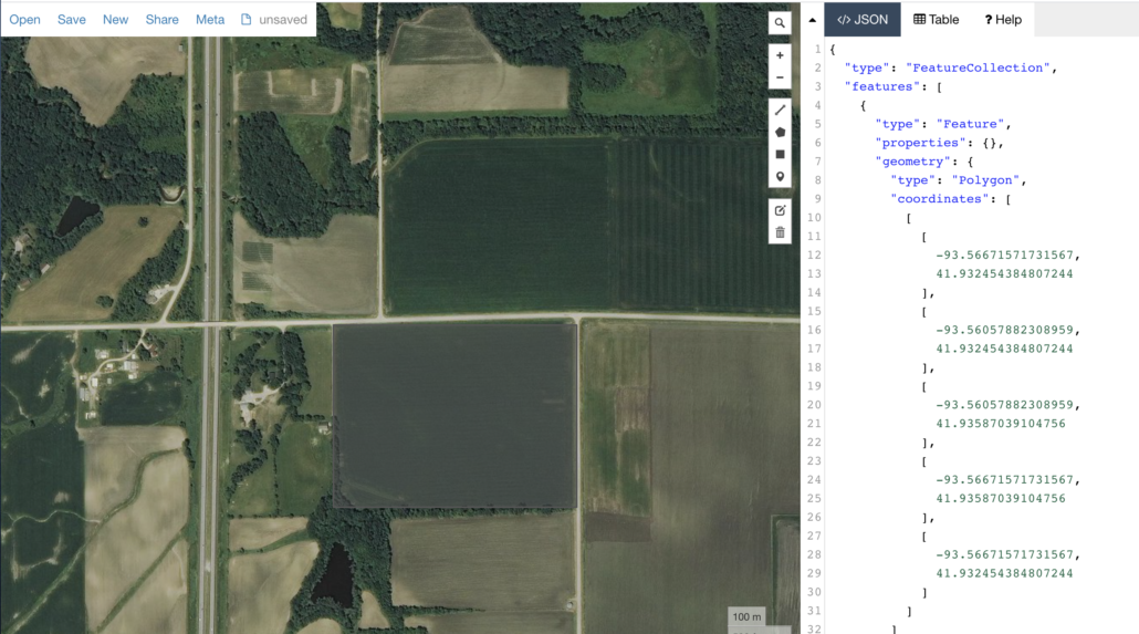
Now that I have my field boundary loaded into HDFS I can use that geometry from the field json file to st_intersects into my Landsat8 table and find the imagery that covers that field. I’m going to pull imagery from all of August so I can see the acquisition dates from right before and after the Derecho hit.
df_field = spark.read.geojson('hdfs://master:9000/geo/input.json')
sqlc.registerDataFrameAsTable(df_field, "field")
field_imagery = sqlc.sql("""SELECT product_id, entity_id, acquisition_date, B4, B5, st_geometry(bounds_wgs84) as geom, (SELECT geometry FROM field) as field_geom
                            FROM landsat_catalog
                            WHERE acquisition_date > to_date('2020-08-01') AND acquisition_date < to_date('2020-08-31')
                            AND st_intersects(st_geometry(bounds_wgs84), (SELECT geometry FROM field))
                            ORDER BY acquisition_date ASC
                          """)
field_imagery.show()
// output
+--------------------+--------------------+--------------------+--------------------+--------------------+--------------------+--------------------+
|          product_id|           entity_id|    acquisition_date|                  B4|                  B5|                geom|          field_geom|
+--------------------+--------------------+--------------------+--------------------+--------------------+--------------------+--------------------+
|LC08_L1TP_027031_...|LC80270312020215L...|2020-08-02 16:59:...|https://s3-us-wes...|https://s3-us-wes...|POLYGON ((-95.944...|POLYGON ((-93.566...|
|LC08_L1TP_026031_...|LC80260312020224L...|2020-08-11 16:53:...|https://s3-us-wes...|https://s3-us-wes...|POLYGON ((-94.349...|POLYGON ((-93.566...|
|LC08_L1TP_027031_...|LC80270312020231L...|2020-08-18 16:59:...|https://s3-us-wes...|https://s3-us-wes...|POLYGON ((-95.941...|POLYGON ((-93.566...|
|LC08_L1TP_026031_...|LC80260312020240L...|2020-08-27 16:53:...|https://s3-us-wes...|https://s3-us-wes...|POLYGON ((-94.363...|POLYGON ((-93.566...|
+--------------------+--------------------+--------------------+--------------------+--------------------+--------------------+--------------------+
Until Next Time….
Next time we will use our new found Landsat files that cover this field to calculate the NDVI using the build in function rf_normalized_difference, and we will see what other trouble we can get into. It’s truly amazing to have the power of Apache Spark working on geospatial data… using SQL. It turns out rasterframes is easy to install and setup, the documentation is great. Being able to work with DataFrames and SQL on-top of geospatial levels the playing field to an otherwise difficult and hard to approach area.